“If you know the enemy and know yourself, you need not fear the result of a hundred battles. If you know yourself but not the enemy, for every victory gained you will also suffer a defeat. If you know neither the enemy nor yourself, you will succumb in every battle.”Sun Tzu
IIntroduction
Modern financial forecasting systems operate over a profoundly diverse information landscape with a wide variety of data types and structures. This creates a massive dislocation between time, accuracy, and the formation of market prices derived from extensive parties.
Energy markets operate similarly, though it consists of physical dynamics and delivery systems, creating a volatile market shape. The underlying complexities include macroeconomic, microeconomic, fundamental, and interconnected relationships regarding the internal structure of energy commodities and sources. In addition to the complexities, weights of importance regarding influence are constantly dynamic.
Classical methods of analysis fall short of effectively transpiring this information on a consistent basis. The vast array of data composition combined with the consistently changing values creates the inability to truly define what is expected of the market.
Incorporating a constellation of methodologies, comprised of non-linear, linear, textual, and qualitative data can create a robust system of predicting and analyzing the duration, magnitude, and direction of energy price movements.
The following system provides a technical overview regarding the development of autonomous infrastructure that allows for the improved accuracy of market dynamics, and provides insight into the overlooked relationships and patterns that exist within the energy domain, creating new investment opportunities, ideas, and innovation.
Though the primary effort was to improve underlying analysis capabilities, the system resulted in creative strategy development, revealing hidden energy dynamics and edge.
Important Note. Claude Code and other large language models helped develop the syntax, infrastructure, and recommendations for machine learning components, including mathematical representations.
IIStack
II-ACloud Autonomy
What cloud autonomy means.
The firm operates with a fully autonomous structure. No manual execution exists regarding the data ingestion, analysis, and output other than the aspect of interface and potential to place positions (which is built out to be autonomous once turned on). The system works within itself, communicating with external APIs and data safely, whilst also running machine learning inference and reasoning layers with large language models through cloud-native design components.
This is feasible considering the components that the cloud provider offers regarding serverless functions, event buses, object storage buckets, container orchestration, and everything in between allowing for systematic cohesion.
The physical layer — what a data center actually is.
Regarding the specifics on how the cloud provider operates these without compromising security when communicating with external data sources includes using multiple core components. The utilization of “cloud” technology becomes readily more reliable and available compared to owned hardware.

Event Bus Components.
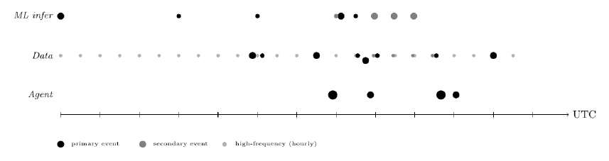

Providing context regarding the core components of this system. The event bus is a scheduling engine that allows for specific enabling of actions / calls without human action. Every action within the system refers back to a specific time and period set by these rules, which occurs autonomously.
Serverless Functions.
A serverless function provides actions without streaming servers, allowing for accurate results and limited latency (~10ms). The hardware is provided by the cloud provider, provisioning micro-VM (virtual machine). This loads the function code or container image at exceptional speeds, and limits the amount of compute consumed between runs.
Object Storage Components.
Object storage acts as the database for the entire system. There is no relational database, no cache, no message queuing system that exist within the system. Every serverless function reads specific data from the object storage and writes output back to different locations within. This makes the system stateless at the compute layer, meaning any serverless function can fail and be retried without corrupting external functions or objects.
The object storage component is organized into several distinct uses, regarding specific machine learning outputs, raw data inputs, and providing context into derived calculations, equations, etc. This component acts as the center of the system regarding any specific data.
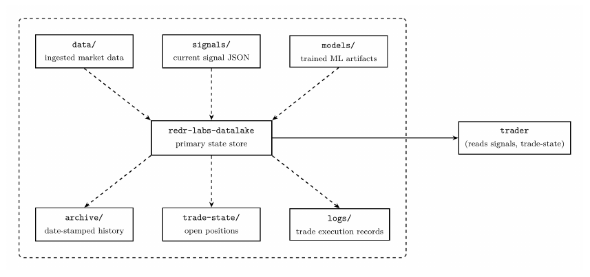
The full autonomous loop.
The components regarding the event bus, serverless functions, and object storage are specific and integral parts into how this system operates fully autonomously. They each serve their purpose, combining into a single continuous loop that runs consistently and precisely to limit interruption.
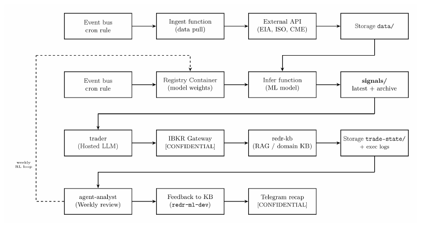
Why autonomy matters.
Regarding the importance of autonomous utilization concludes with several advantages. Speed / reaction latency are far more advanced versus manual pulling, though the core advantage stems from consistent, tireless execution on every invocation, whilst also enabling to scale by pulling from different data sources at the same time.
II-BData Ingestion Architecture
Specific Detail.
The serverless functions issue an authenticated HTTP GET to the external data provider, which typically returns a JSON or CSV formatted data / dataset. The function parses and validates the response and provides a timestamped file to its assigned prefix or appends to a specific file for additional processing. The infrastructure runs over 50 serverless functions in total across data ingestion.
Daily Ingest Volume.
Assuming the data is depicted within a CSV, let ri be the row count per invocation of function i, where fi represents the daily firing count, and b ≈ 120 bytes (120 bytes is the average row size for a typical energy time-series CSV). Total daily ingest volume:
Depending on the day interval and payload, ri ∈ [24, 288] rows, which is representing a typical hourly or five-minute ISO data pull. Where, the volume per day or Vday falls within the range of [10 MB, 80 MB]. This is well within the object storage limitations regarding storage amounts. (∈ represents an element of, 24 for hourly, and 288 for 5min interval daily). That represents 288 data points per day from one Independent System Operator (ISOs) data type (DAM LMP 5min).
II-CData Cleaning Processes and ETL Framework
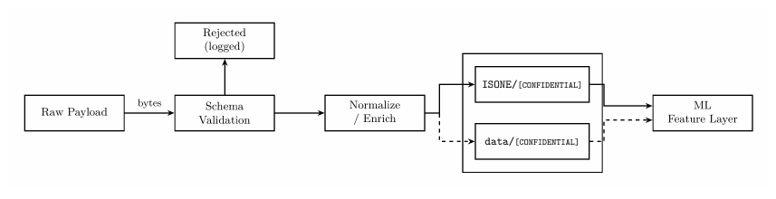
Extract, Transform, Load (ETL) pipeline.
The ETL layer transformed raw API responses into the numerical feature types that are able to be readily utilized by ML models. It operates across six structural stages.
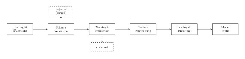
Schema validation and imputation post data ingestion.
Before any feature is computed, each ingestion of data is validated against a specific data schema, which is essentially what the data is expected to look like. This includes the field names, timestamps, numeric columns, labels, etc. Invalid payloads are rejected. Once verified valid, two specific classes of imputation / cleaning are applied:
Forward Fill. Missing daily observations such as holiday closures during weekdays or API gaps, are filled from the previous valid value. This preserves the continuity of the rolling windows regarding machine learning platforms.
Winsorization. For extreme outliers, which include values beyond the 1st and 99th percentile of the trailing 252-window, they are clipped to a boundary value prior to scaling. This prevents a single bad API response from blowing out a StandardScaler fit, or misrepresentation.
Feature construction.
Raw field values are combined and derived into different features that represent relationships. These features are then consumed by the machine learning models. Specific derived values include:
| Feature | Derivation | Consumed by |
|---|---|---|
| Thermal Generation % | [CONFIDENTIAL] | GMM, triple indicator |
| Natural Gas Generation Share % | [CONFIDENTIAL] | GMM, LSTM, MAS AE |
| Natural Gas Spread | [CONFIDENTIAL] | LSTM AE, spread model |
| Natural Gas Spread % Change 1d and 5d | [CONFIDENTIAL] | LSTM AE |
| Heating Degree Day Deviation | [CONFIDENTIAL] | GMM, LSTM |
| Heating Degree Day Z-score | [CONFIDENTIAL] | MAS AE |
| Petroleum Burn | [CONFIDENTIAL] | MAS AE |
| PADD1 Distillate | [CONFIDENTIAL] | MAS AE, spread model |
| Crack Spread | [CONFIDENTIAL] | Neural ODE (γ coeff) |
| Storage Deficit | [CONFIDENTIAL] | GMM, Neural ODE |
| Volatility Z-score | [CONFIDENTIAL] | Triple indicator |
Table I. Derived feature construction used across the ISO machine learning pipeline.
StandardScaler.
StandardScaler, is applied to the continuous feature vectors prior to LSTM and GMM layer entry. The function maps each feature to zero mean and unit variance:
Where μ̂ and σ̂ are estimated from the training window and serialized (.pkl file type) alongside model weights. The rolling z-score is the inference-time analog of StandardScaler:
Where zt represents the rolling z-score, xt is the current observation, μ30d is the 30 day rolling baseline mean, and σ30d represents the 30 day rolling standard deviation. This is the direct mechanism in which the system makes today’s observation comparable across time, providing context by derived values within history. The same raw LMP value is interpreted differently in summer and in winter once normalized to its recent context.
Why this matters for LLM autodetection.
A StandardScaler is fitted within a dataset with a distribution shift (e.g. post-COVID demand collapse, or gas price spike) will produce systematically biased z-scores. The output will be dictionary meaningful but shifted.
OneHotEncoder.
OneHotEncoder is the methodology for representing categorical values as numerical values, without skewing them with bias due to invalid weight contexts. The variables that they are applied include:
| Categorical variable | Levels | Used by |
|---|---|---|
| ISOs | ISONE, ERCOT, CAISO, NYISO, MISO, PJM | MAS 119-feature AE, VGAE |
| Fuel Types | gas, coal, nuclear, hydro, wind, solar, oil | GMM fuel-mix feature |
| Regimes | 0, 1, 2 (learned GMM labels) | LSTM input, agent context |
| PADD Regions | PADD1, PADD2, PADD3, PADD4, PADD5 | Petroleum feature layer |
| EDGAR Sector | E&P, midstream, refining, utility (10 sectors) | EDGAR signal aggregation |
Table II. Categorical variables and their one-hot encoded levels.
The encoding represents a single categorical column into k binary columns, which allow for accurate training of machine learning models. Where the values are binary, no false weights are provided as anything greater than 1, has bias versus the value of 1 or 0.
Example if gas was the primary fuel type looks like the following:
| fuel_type_gas | fuel_type_oil | fuel_type_wind | fuel_type_solar |
|---|---|---|---|
| 1 | 0 | 0 | 0 |
Table III. One-hot encoding example if gas was the primary fuel type.
Whilst if solar was the primary fuel type:
| fuel_type_gas | fuel_type_oil | fuel_type_wind | fuel_type_solar |
|---|---|---|---|
| 0 | 0 | 0 | 1 |
Table IV. One-hot encoding example if solar was the primary fuel type.
Drop-first convention.
To avoid dummy variables, the first level of each category is dropped. The GMM and LSTM remain unaffected since they operate on the full feature vector without an intercept, but the LightGBM spread model uses the drop=[first] by convention.
Seasonal cyclical encoding. The stacked LightGBM spread model encodes month and week_of_year as sine-cosine pairs rather than one-hot vectors. This preserves the cyclical continuity that one-hot encoding would perhaps break.
II-DOperations Infrastructure, Front-End Platform
Platform overview.
The Operations Infrastructure is the operator-facing web platform for the technical stack. It surfaces the entire ML and LLM pipeline as a usable interface, including live AI market analysis, autonomous trade execution controls, position monitoring, signal visualization, data exploration, and agent management. The platform is built on Next.js 16 with the App Router, deployed to Vercel, and maintained within a private GitHub repository. Every push to the main branch then triggers a Vercel Continuous Integration (CI) build. There is no separate build or deployment infrastructure, serverless API routes handle all communication between the cloud infrastructure and the Operations Infrastructure.
Application shell and navigation.
| App | Function |
|---|---|
| Ops | AI analyst chat, trade controls, signal hub |
| Command | React Flow canvas, ESS project appraisal |
| My Agents | Agent config, app builder, dataset browser |
| Dashboard | P&L overview, weekly reports |
| Data | Object storage browser, cross-signal correlation, CSV upload |
| Positions | Live IBKR positions, trade history |
| Charts | UNG, USO, BNO candlestick + spread charts |
| Scan | Multi-signal market scan |
| Cycle | Manual agent cycle trigger |
Table V. Application shell and navigation.
energyOS — the AI analyst interface.
energyOS is the primary interface. It is a streaming chat that assembles a prompt from 40+ parallel object storage reads, passes it to Claude Sonnet via the managed foundation model API, and renders the streamed markdown response in real time.
Authentication.
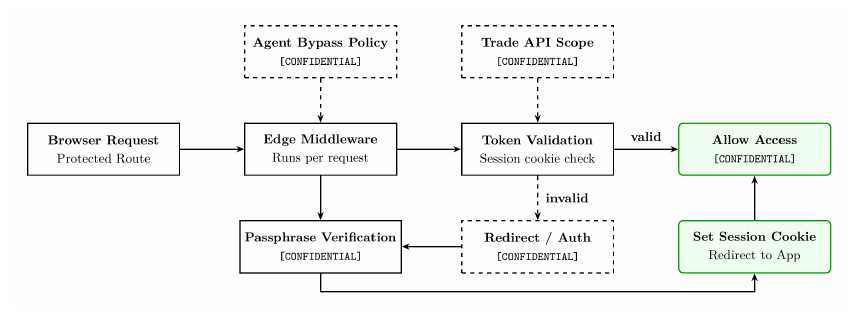
Operations Infrastructure uses a custom passphrase-based authentication system with over 20 characters. No OAuth provider is required, access is controlled by a list of passphrase strings configured as a Vercel environment variable and are never shown to any public facing data.
| Library | Version | Used in | Purpose |
|---|---|---|---|
| mapbox-gl + react-map-gl | 3.22 / 7.1 | MapDashboard | Base tile layer for geospatial views |
| @deck.gl/layers | 9.3.1 | MapDashboard | Hexbin, scatter, arc layers over Mapbox for satellite signal viz |
| @react-three/fiber + three | 9.6 / 0.184 | 3D views | WebGL 3D scene graph, signal topology visualization |
| recharts | 3.8.0 | Analytics, Hub | Standard bar, line, area charts for signal dashboards |
Table VI. Main visualization libraries.
The deck.gl layer runs on top of Mapbox, rendering PADD3 refinery site information as a heatmap and satellite thermal signals. Three.js is used for signal topology view, which directly renders the cross-commodity graph as a 3D directed network.
Key dependencies and runtime.
| Package | Version | Type | Role |
|---|---|---|---|
| next | 16.1.6 | prod | App Router, API routes, Edge middleware |
| react + react-dom | 19.2.3 | prod | UI rendering |
| typescript | 5.x | dev | Type safety across all source files |
| tailwindcss | 4.x | dev | Utility CSS, PostCSS pipeline |
| Object storage SDK | 3.1011 | prod | Object storage reads from API routes |
| Foundation model runtime SDK | 3.1036 | prod | Claude inference |
| Key-value store SDK | 3.1034 | prod | Session/usage tracking |
| Serverless invoke SDK | 3.1047 | prod | Invoke agent serverless functions |
| Telemetry & metrics SDK | 3.1047 | prod | Pipeline health metrics |
| Email service SDK | 3.1055 | prod | Email notifications |
| @vercel/analytics | 2.0.1 | prod | Page-level analytics |
| papaparse | 5.5.3 | prod | CSV parsing for user uploads |
| lucide-react | 0.577 | prod | Icon set |
| playwright | 1.60 | prod | Headless browser automation |
Table VII. Key dependencies and runtime.
Data ingestion panel — user-uploaded signals.
Operations Infrastructure allows for the uploading of datasets that are analyzed in-browser and provided into chat context. This adds another layer of adaptability regarding signal research and learning. When data is uploaded via the panel, for example a csv, PapaParse parses the file in the browser, then the system auto-detects the data columns, trend region and residual uncertainty bands are computed, z-scores included. The LLM treats the uploaded data as main signals alongside the existing pipeline outputs.
Security Properties.
The front-end has specific security properties by design. These include the following:
- No Credentials in the Browser. All cloud SDK calls occur within the Next.js API routes, server-side. The browser only fetches from the Vercel endpoints.
- Three Distinct Authentication Surfaces. Separate secret functions to eliminate compromise across other endpoints.
- Atomic Use Limits. Managed key-value database conditional enforcement of passphrase usage caps with no race condition.
- Read-Only Identity and Access Management. Vercel’s cloud credentials are scoped to read operations on a specific location via ARNs, the front-end cannot write to any of the internal systems or invoke operations such as serverless functions or modify any cloud components.
- Private Repository. Source code, including all front-end deployments are within a private GitHub repository with no public fork.
IIIComponents
III-AIndependent System Operator Inference & Training Pipeline
Overview.
Regarding the ISO pipeline, it comprises several serverless functions, covering ISONE, ERCOT, CAISO, and NYISO. Each function runs from the same container registry image, ~[CONFIDENTIAL], built per ISO, with the operating mode controlled by an environment variable.
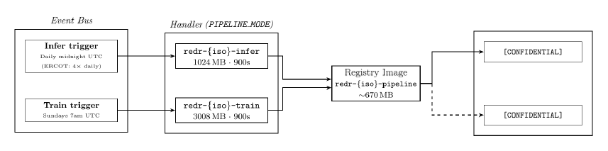
Input data.
Each function reads a consistent set of inputs from the object storage before running, whilst the container resolves the correct path based on the ISO identifier.
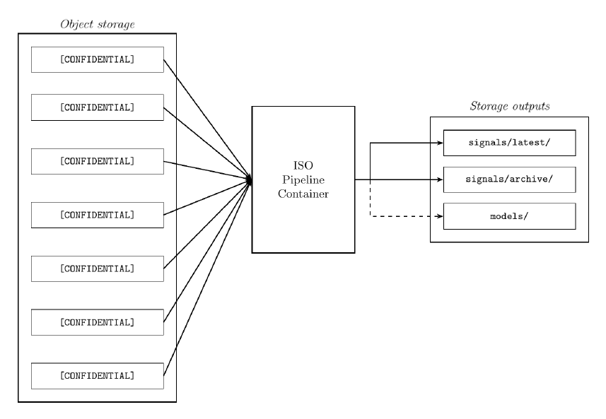
How the Machine Learning Pipeline Works.
Instead of predicting electricity prices using linear regression formulas, the pipeline detects grid stress regimes. The structured operational states in which the relationship between grid generation mix and natural gas prices becomes statistically exploitable / predictable.
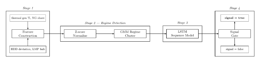
Step 1 — Z-score normalisation.
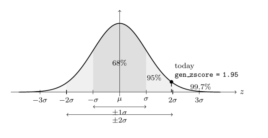
Prior to any model sees the data, each raw feature x becomes normalized against its own recent history using a rolling z-score:
μw and σw are the mean and standard deviation computed over the trailing w = 30 trading-day window. A z-score of 0, represents the central part of the normal distribution, exactly the recent average. A z-score of +2 represents two standard deviations above the mean, which would be unusual. Examples of this include unusually high thermal generation, or large natural gas electricity generation share. This is how the model can detect unusual activities that are occurring with the grid.
Step 2 — Gaussian Mixture Model regime detection.
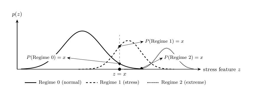
After normalisation utilizing z-scores, a Gaussian Mixture Model (GMM) assigns today’s feature vector to one of K learned market regimes. Regime amounts are represented by the amount of K values. The GMM models the overall distribution of historical grid states as a weighted sum of K Gaussian components:
Each component k has a mixing weight πk or how often the market is within that state, a mean μk represents what the regime looks like, and a covariance Σk shows the range or how spread out it is. At the inference time, the model computes the probability that today belongs to each regime and assigns the label of the most likely one.
Step 3 — LSTM sequence model.
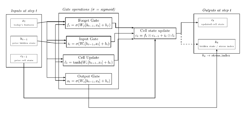
Energy data is sequential, today’s grid configuration depends on yesterday’s generation dispatch and last week’s EIA storage number, and temperature trends that are typical during the present season, etc. A standard feedforward network ignores temporal structure. An LSTM maintains a cell state c that acts as long-term memory, updated at each time step through the three learned gates (Forget, Input, and Output).
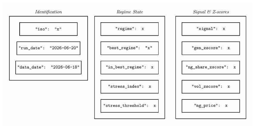
Signal output.
Both the inference that occurred along with the edge-signal functions write a single JSON file, overwriting the previous run on each execution:
III-BMachine Learning: Unsupervised & Signal Models
Function 1 — Unsupervised Machine Learning.
Overview. The model runs three times daily and has no labeled training targets, representing the unsupervised aspect. It combines four distinct techniques into a single inference pass, these include:
- LSTM autoencoder that learns what normal market structure looks like and flags deviations.
- Causal entropy tracker that measures the amount and what are the active physical drivers.
- A topological data analysis (TDA) module that monitors the shape of correlation across all datapoints.
- A neural, ordinary differential equation that models price dynamics using physical coefficients.
The main premise of these functions are to identify patterns of correlation and impact that exist within the data, allowing for detailed assessment and understanding of relationships in price action. Memory: 1769 MB. Timeout: 600s.
LSTM Autoencoder.
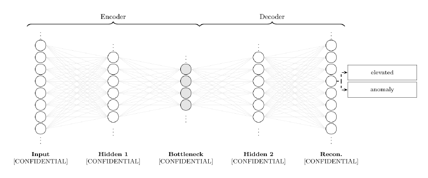
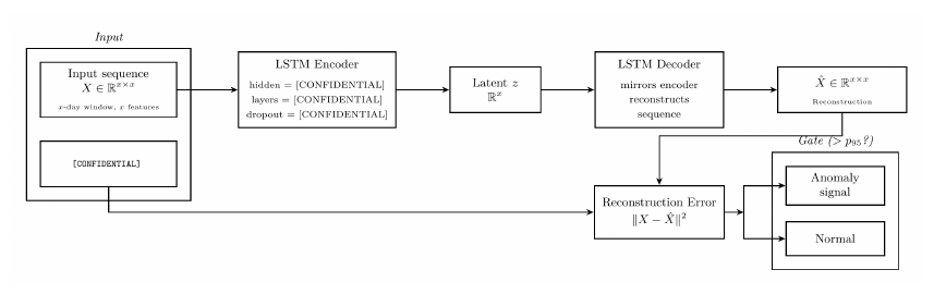
Regarding what an autoencoder is, it learns how to compress data to a low-dimensional representation and then reconstruct it. The model itself is trained exclusively on normal market data, therefore, at inference time with real conditions applied, anomalous inputs such as conditions that are unseen produce larger reconstruction error which provides an anomaly signal. This acts as a signal inference for unseen conditions or things the model potentially has not expected.
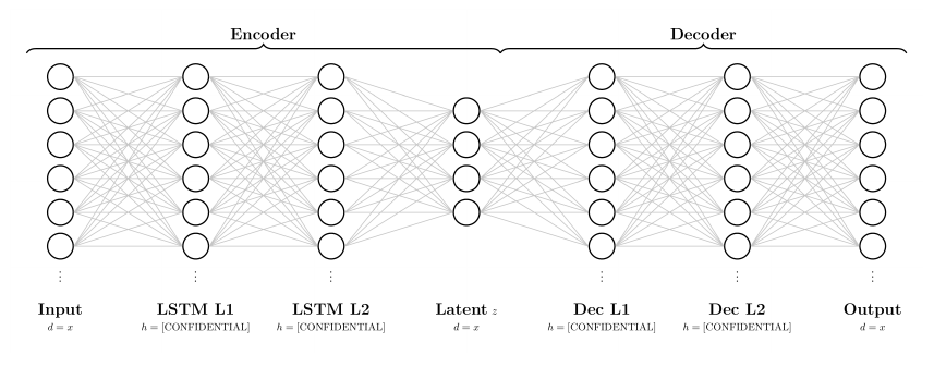
The autoencoder uses a Long-Short Term Memory (LSTM) to process a rolling window of [CONFIDENTIAL] across [CONFIDENTIAL] features. These are then compressed into a 16-dimensional vector, then the decoder reverses this, attempting to reconstruct the original sequence.
Regarding the specific nature of how a neuron works, each input represented by xi is multiplied by a learned weight wi, summed with a bias represented by b, then passed through a nonlinear activation function σ. Without each nonlinear component, every layer would collapse into a linear map which then stacks layers and adds nothing. The nonlinearity allows the deep networks to learn untraditional patterns. The weights and bias values are learned through a gradient descent methodology.
A second, larger autoencoder (mas_autoencoder.pt, 3.5 MB, trained May 17 2026) compresses [CONFIDENTIAL] simultaneous market features — spanning all five ISOs, petroleum, NG, weather, and satellite signals — to a [CONFIDENTIAL]-dimensional bottleneck. This has [CONFIDENTIAL] input features, named “MAS” or Market Aware System.
Function 2 — Causal Entropy.
Entropy is another word for uncertainty.
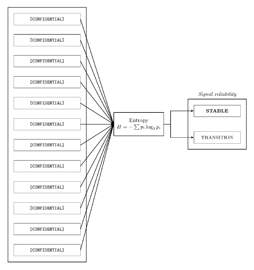
The model analyzes [CONFIDENTIAL] causal pathways between physical market drivers and the corresponding price points. Each pathway has an activation probability pi which represents the strength of how that driver is influencing the price at a specific timestamp. Shannon entropy over these probabilities measures overall market clarity in price formulation.
Shannon Entropy. H represents the entropy, pi represents the probability of an outcome, log2 represents the measurement of entropy in units of bits, and Σ represents the sum of all possible outcomes in this system.
The amount of low entropy reveals that one or two drivers are dominating market pricing, representing a clear, physical cause. Higher entropy represents that many drivers are actively impacting at the same time, which tells that the system is in a transitional / confused state.
Function 3 — Topological Data Analysis (TDA).
Literally creating a physical shape of the data.
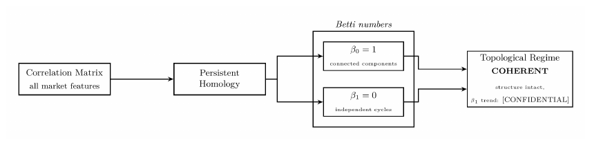
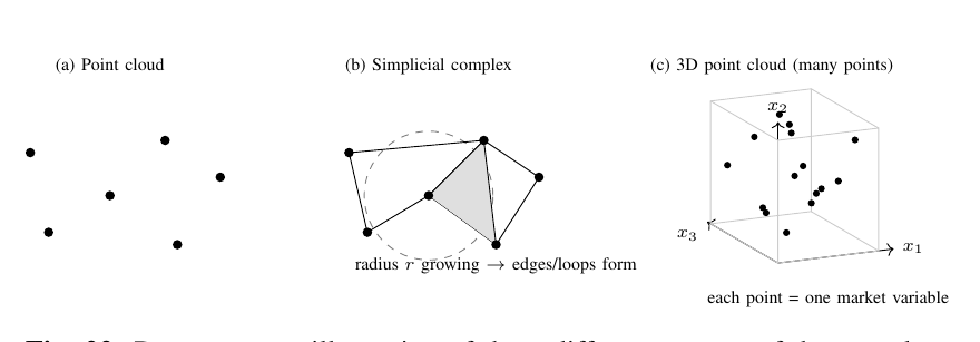
The TDA measures the shape of the correlation matrix across all of the market variables, using tools from algebraic topology. The key aspects of technical framework include Betti numbers which β0 counts the number of disconnected components in the correlation graph, and β1 counts the number of independent cycles or loops within the graph. A cycle appearing in the correlation structure represents a set of assets mutually reinforcing components within a closed loop. This shows a classic signature of structural stress. When β1 > 0 and persistence entropy is rising, the topology becomes more complex, which shows instability before it is represented in pricing. Complexity of topology is the measure of instability which can be used to predict pricing.
Component 4 — Neural Ordinary Differential Equations (ODE) (fair-value dynamics).
A neural network that conducts flow as opposed to consistent breaks / points of structure.
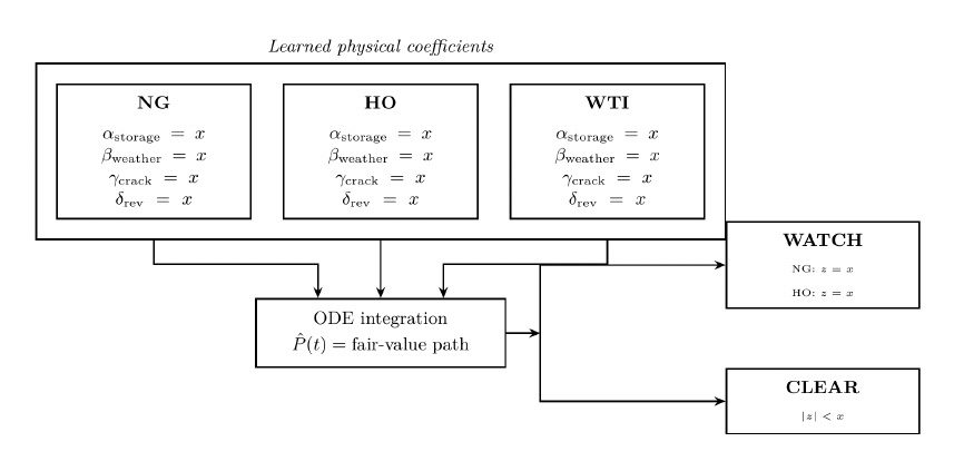
A neural ODE models actual price dynamics using a continuous differential equation rather than a discrete time step. For each commodity (NG, HO, WTI) the model learns physically interpretable coefficients that govern how price evolves / is formed over time:
d(log P)/dt represents instantaneous growth rate, which is equal to that of α weight for storage, β weight for weather, γ weight for the crack spread, δ representing the mean-reversion force that is pulling the price toward a learned value or speed of adjustment, and εneural represents the neural network residual, complex adjustment.
A good analogy represents that of the classical terms (α, β, γ, and δ) as the predictable smooth components like a predictable highway of where the price should go based on fundamentals. Whilst the neural network residual εneural acts like minor steering wheel adjustments for correcting wind, road texture, and traffic on the highway.
III-CSatellite Signal Models
Model Data.
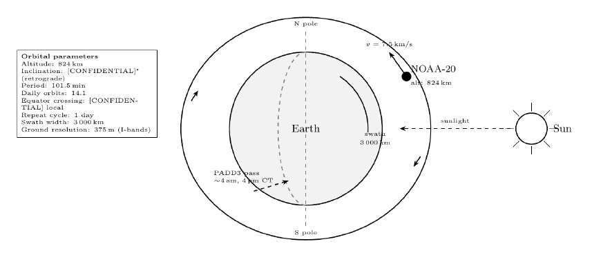
Both models are driven by NASA’s FIRMS (Fire Information for Resource Management System) API, which distributes thermal anomaly detections from the VIIRS instrument (Visible Infrared Imaging Radiometer Suite) aboard NOAA-20 (formerly JPSS-1). Refineries are dark, but their process heat is not, and spotted with thermal infrared and surface temperature measurements.
NOAA-20 and the sun-synchronous polar orbit.
The NOAA-20 flies in a sun-synchronous, near-polar orbit (SSO). This represents a low-atmospheric orbital that allows for the satellite to pass by a specific location everyday at a consistent time. Regarding the equator, the satellite always crosses at the same time, 01:30 descending and 13:30 ascending. This guarantees a consistent solar illumination of geometry for every pass, which remains critical for measuring and removing solar-heat bias from surface temperature retrievals.
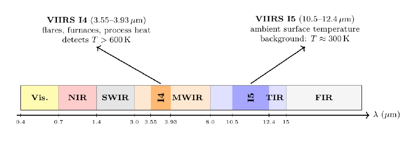
Electromagnetic spectrum and VIIRS detection bands.
The VIIRS instrument has 22 spectral bands that span 0.41 to 12.5 micrometers (µm) or one-millionth of a meter. Two imagery bands are critical for energy infrastructure monitoring, they are the I4 and I5. I4 detects hot targets which include gas flares, furnaces, and processing heating radiating from the refineries above ~600K and measuring between 3.55 through 3.93 µm which represents mid-wave infrared. I5 measures ambient surface temperature and is used to compute the background from which I4 datapoints are isolated. I5 acts as the control variable to provide a reference point for the I4 measurements. I5 measures around 10.5 to 12.4 µm. Where .7 µm is visible to the human eye and over 4,000K.
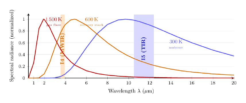
Planck radiation: why hot sources glow in the infrared.
Every object that is above absolute zero emits thermal radiation, which this principle can be described within Planck’s law as spectral power emitted per unit wavelength:
h represents Planck’s constant, c is the speed of light, k is Boltzmann’s constant, T is temperature represented within Kelvin, and λ is wavelength. There is an aspect of temperature impact regarding peak shifts represented by Wien’s displacement law:
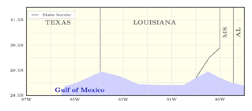
PADD3 geographic coverage.
Across the United States, there are five distinct locations of Petroleum Administration for Defense Districts (PADDs) used to track crude and refined goods. PADD3 serves as the hub for the production of these energy resources across the United States. PADD3 is large, located in the Gulf Coast. The model monitors 25 sites across this area, spanning from Texas, Louisiana, Mississippi, and Alabama. Each site has a bounding box via coordinates, in which VIIRS pixels falling within the box are attributed to that site and aggregated to daily amounts.
Machine Learning via PADD3 Satellite.
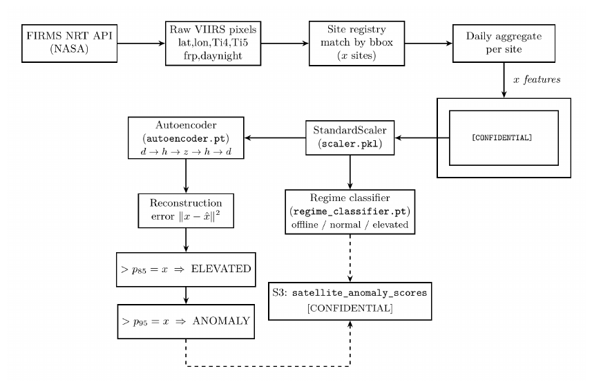
Everyday, the serverless functions via the event buses call the FIRMS NRT (Near Real-Time) API with the prior day’s data, and receives all of the VIIRS I4 detections within each site’s bounding box, and aggregates them to per-site daily features, and then runs an inference through two models: A tabular autoencoder for anomaly detection and regime classification system for operating state labeling. These functions are similar to the ones shown in Figure 8.
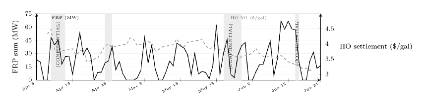
PADD3 fire radiative power vs. heating oil price.
Refinery activity is a direct physical input to distillate supply. When throughput surges (high FRP, many detection events), more heating oil and diesel is being produced. When throughput collapses (zero FRP, no thermal signal), unit outages or planned maintenance may be tightening supply.
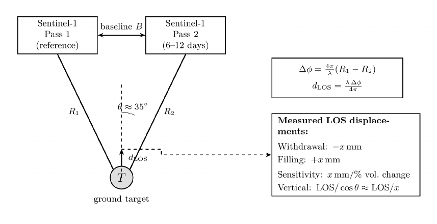
Synthetic aperture radar and InSAR ground deformation.
Whilst the VIIRS instrument remains effective for detecting surface thermal emissions, a second technique, Synthetic Aperture Radar Interferometry (InSAR) measures the physical movement of a ground surface. The instrument measures the ground surface deformation above underground storage caverns with millimetre precision. A specific SAR satellite, the Sentinel-1, uses its C-band (λ = 5.55cm) to illuminate the ground with microwave pulses and records complex backscatter phasing. The difference between the phase of two passes separated by days to weeks gives the line-of-sight (LOS) displacement:
Where Δϕ represents the difference, (4π/λ) shows one 2π fringe = λ/2 = 5.55/2 = 2.775cm LOS displacement and dLOS represents dvertical·cosθ + dhorizontal·sinθ for satellite incidence angle θ of ~35°.
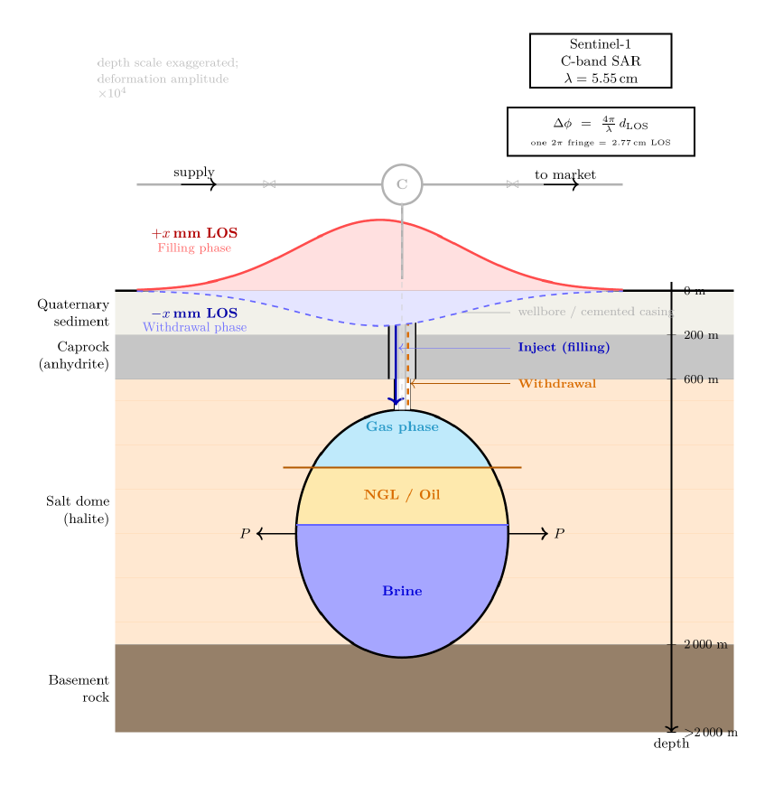
Deformation Metrics.
The salt domes of the Gulf Coast are massive bodies of halite (NaCl) that pierced overlying sediments over millions of years, their impermeability and mechanical strength make them ideal for underground storage. They are used to store gas, oil, or brine, by being injected under pressure and held indefinitely.
Peaker Plant Monitoring.
The ERCOT model monitors [CONFIDENTIAL] natural gas peaker and combined-cycle turbine plants across Texas, correlating their thermal signature with gas generation share via public data. When large peaker plants show elevated FRP, gas demand on the ERCOT grid is high, which tightens Henry Hub natural gas prices. The model output assigns specific dispatch labels. The natural gas, electricity-generation share provides an external supervision signal, allowing the model to distinguish structural high-dispatch periods from anomalous plant restarts.
Compound Learning.
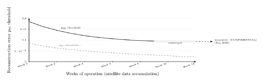
Both of the satellite models retrain autonomously at specific periods, regarding weights. This is to align with policy, macro, and subsects of catching decay. Each retraining cycle ingests all accumulated site-days and re-fits the autoencoder, updating the thresholds from the new error distribution. This is the same function for the classifier as well. Early in development and creating real time predictions, the model has little history and anomaly thresholds are set from a historical distribution. As months of real time data accumulate in real time, the percentile thresholds become more accurate, where the false-positive rate drops, and can determine rare / genuine anomalies more effectively.
Triple Indicator ML System
What it does.
This model runs daily and produces edge signals, which present the core per-Independent System Operator (ISO) trading signal used by a large language model (discussed later). It is called the triple indicator system because the stress index is developed from three independently computed z-scores, each measuring a different dimension of grid stress.
The three indicators.
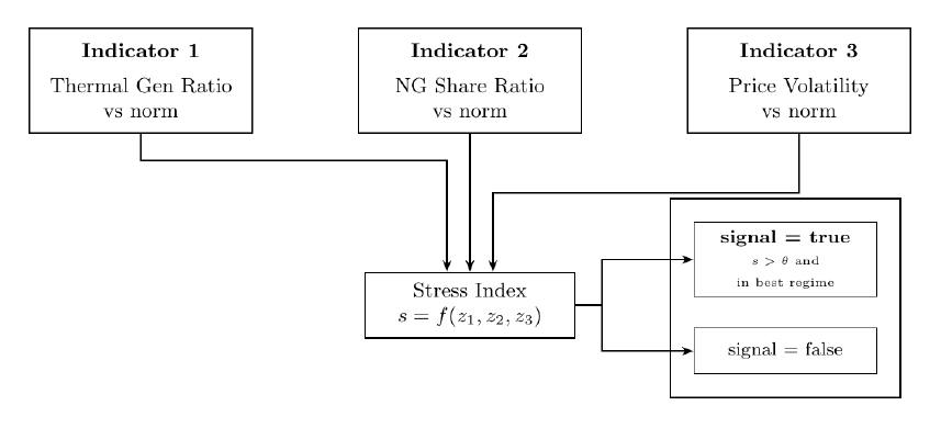
Firstly, is the grid running unusually high on thermal generation, is the natural gas share of the fuel mix unusually high, separate from the overall thermal, and are the locational marginal prices (LMP) for [ISO] elevated with volatility? The LMPs spiking consistently provides insight that the grid operator is struggling to balance supply.
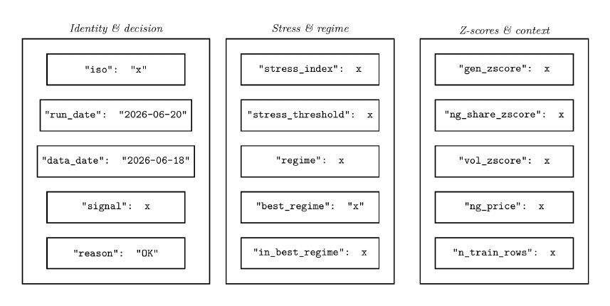
Output record.
Market Spreads ML
What it does.
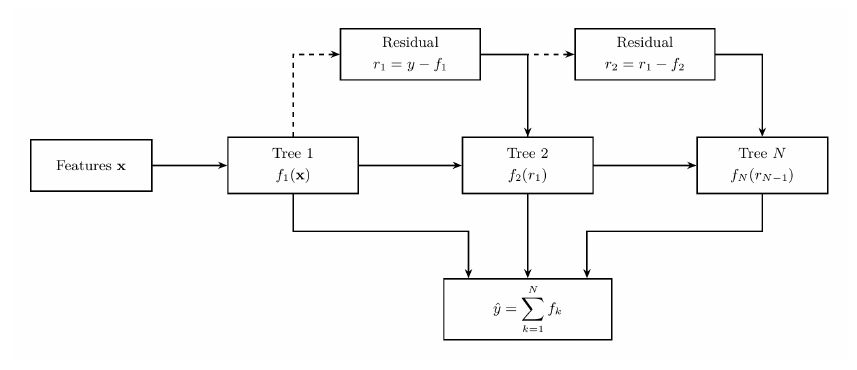
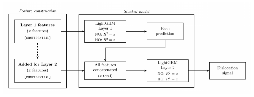
Running daily on weekdays, the model predicts whether the natural gas–heating oil and natural gas–crude oil spreads are dislocated from their physical comparative fair values. It is a two-layer stacked model, with the first stage generating a base prediction and the second stage refining it by adding spread-specific features such as lag, momentum, etc. in which the first stage is blind to. Both stages use LightGBM which are gradient boosted decision trees (unsupervised learning) trained on model artifacts that live with the object storage data lake.
LightGBM – Use Case.
LightGBM builds an ensemble of decision trees sequentially, each tree corrects the residual errors left by the previous trees, where the final prediction is the sum of all of the trees’ outputs.
Construction of the Two-Layer.
III-Dagent88 — Novel Signal Generation, Entropy, and Continuous Dynamics
What agent88 is.
Regarding the main ISO electricity models, these models are trained on structured time-series features that arrive on a fixed daily or weekly schedule. The agent88 provides a function via a container that targets the whitespace, signals which were not captured by scheduled ISO data pulls such as corporate hedging behavior, etc. Daily, entropy scans, novel feature synthesis, and signal emission functions are fired. These provide context regarding tradeable thresholds, pipeline nominations that arrived overnight, and textual rationale for reasoning layers.
Signal Quality.
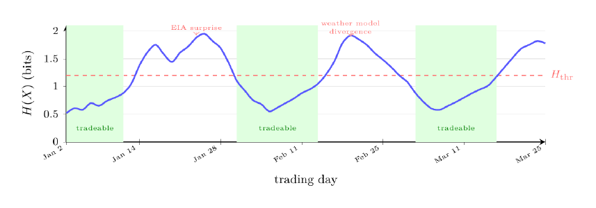
Energy markets are often in high-entropy states, which are noisy, unstructured, and unpredictable due to the sheer multitude of external direction variables. The core of agent88 is that structured low-entropy physical regimes occasionally emerge from the typical noise, and are the only conditions worth trading in the public energy markets. Entropy provides the primary gate in which whether a signal generated is actually feasible to push the market in the predicted direction.
Entropy Over Time.
The gate is established and evaluated daily. Tradable windows are not predictable from the calendar, but rather emerge from physical conditions. High-entropy periods such as EIA surprise print, weather model divergence, and macro impact via geopolitical shocks are skipped entirely.
Mutual Feature Selection.
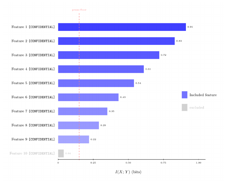
Mutual information measures how much knowing feature X reduces uncertainty about the target of Y:
Where H represents entropy. Features with I(X;Y) below a floor are pruned during model training, whilst energy markets representing high-I features are physically determined. These include storage draws, generation fuel mixes, pipeline nominations, etc.
Entropy Loss for Regimes.
The training objective for all regime classification models is cross-entropy over the K-class output which is represented by:
Where L represents loss, Σi sum over all samples, Σk are the all possible regimes, yik is the one-hot-encoder category represented as binary, 1s and 0s, and p̂ik represents predicted probability that i belongs to class k. Where if yik = 1 and if sample i is truly within regime k and p̂ik is the predicted probability, then minimizing L is equal to minimizing KL divergence between the predicted and true distributions.
Continuous Dynamics v Postings.
Discrete models such as LSTMs and transformers observe energy market state at calendar intervals, though the underlying physical stream is continuous and volatile. These include pipeline pressure, generator ramp rate, storage cavern temperatures, etc.
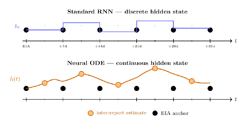
From discrete RNN to continuous ODE.
ODEs provide the bridge between the transition of energy observations, providing them to be continuous. A standard Recurrent Neural Network or RNN updates a hidden state discretely at each time step, whilst an ODE replaces this with a continuous differential equation.
Inter-report state estimation.
Between weekly EIA Natural Gas Storage reports, agent88 uses the neural ODE to maintain daily estimates of working gas in storage, using inputs to inter-report day + physical components.
Evolutionary Model.
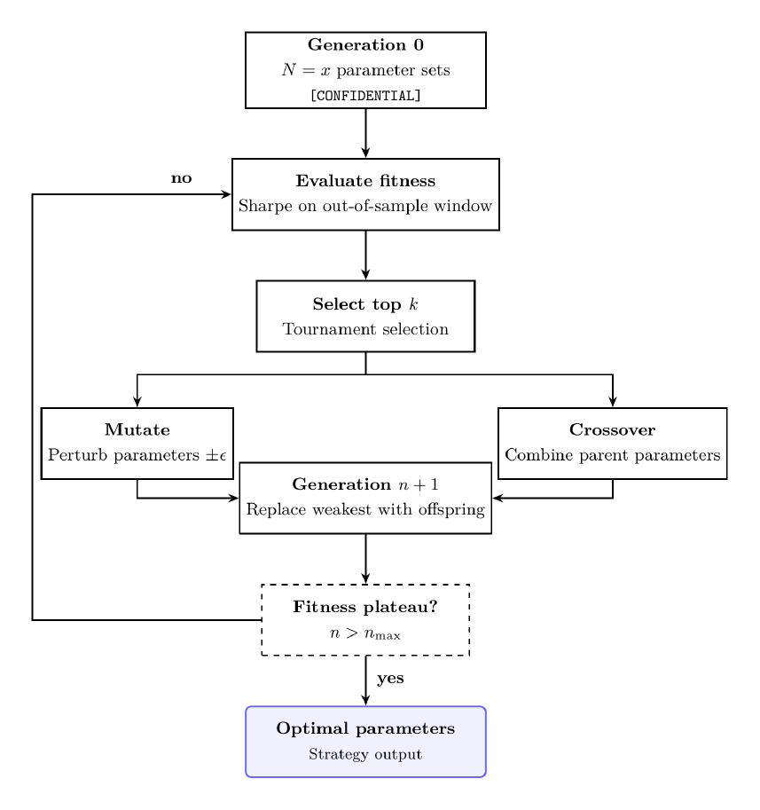
Gradient-based optimization finds good model weights but fails to effectively search for strategy parameters which includes discrete choices. The EVO model applies a genetic algorithm to this problem.
Convergence.
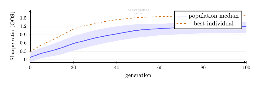
The algorithm typically converges within 60 to 80 generations, where early generations are dominated by random value variation and the crossover begins consolidating high-Sharpe parameter combinations after generation 20 and population median stabilizes above the initial baseline by generation 50.
Kolmogorov-Smirnov drift detection.
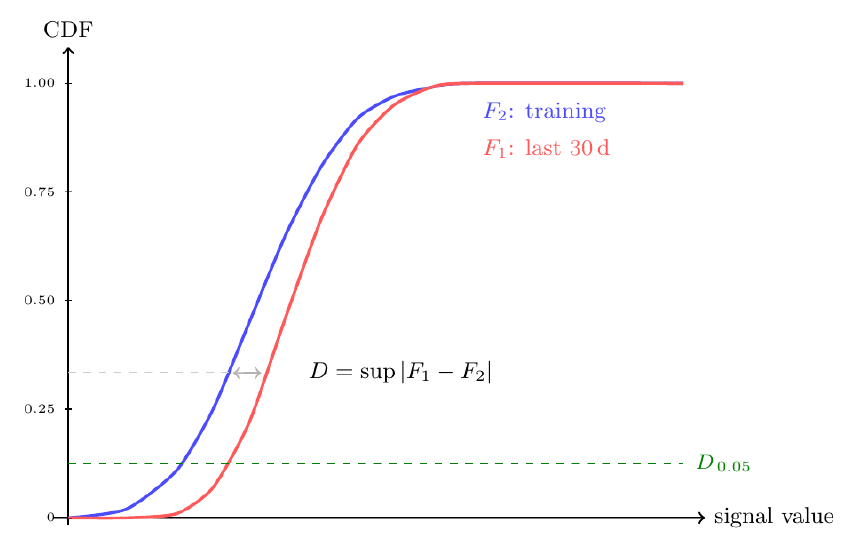
When training models based on historical distributions, it is important to implement some type of market shift analysis considering markets shift structurally. This includes policies by FERC or the DOE, new use of an LNG export terminal, etc. The Kolmogorov-Smirnov (KS) test is the primary mechanism for detecting this.
Two-Sample KS.
The KS statistic compares empirical Cumulative Distribution Functions (CDFs) of two samples:
where F1 is the single CDF over the last 30 days and F2 represents the training CDF. When D exceeds the critical value at p < .05, the distributions are significantly different, and the model shows drift. Probably known from the term “reject the null hypothesis.” Actions are put into place for retraining.
III-EManaged Foundation Model Autonomous LLM Layer, Three-LLM Architecture
Three LLM Architecture.
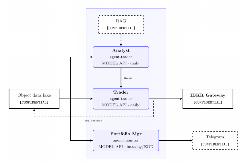
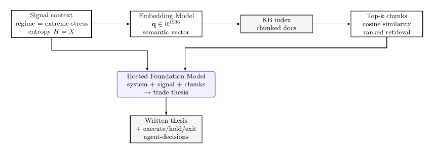
Most algorithmic trading systems are either pure quant, or pure LLM, where both fail at the boundary they ignore. This occurs because pure quant systems cannot assess whether a signal is physically coherent given the macro environment, whilst pure-LLM systems have no structured physical model to prevent hallucinated rationale + lack of quantitative capabilities because LLMs are inherently language prediction models. Combining both and creating a hybrid system proves to be the best approach. The machine learning pipeline / methodology previously discussed, with outputs landed within the object storage. Combining that with the managed foundation model API component, using LLMs to read those structured outputs and provide critical thinking over them in natural language, grounded in early domain knowledge via RAG, proves to be exceptionally high-performing. The result is a written trade thesis that can be read, audited, discussed, before execution happens. Three distinct functions require three distinct communicative LLMs, because they operate on different information at different frequencies, with different risk.
Managed Foundation Model API.
The managed foundation model API is a managed API that exposes foundation models such as Claude, Llama, Nova, etc. without requiring any direct model hosting, GPU provisioning, or weight management.
Three properties are critical for a production priority information market prediction system:
Identity and access management-native security. Serverless functions call the foundation model API via their identity and access management execution role, where no API keys are stored anywhere. No .env files, no hardcoded tokens. The call chain is an event bus trigger → serverless function → foundation model API.
No Data Egress to External Networks. Foundation model API calls using Claude Sonnet 4.6 stay within the cloud provider’s regional boundaries. The input prompt which includes live position data, signal scores, portfolio state, and methodology never accesses the public internet. This is different from calling Anthropic’s API directly, where all inference traffic exits the cloud environment.
Audit Manager Integration. Every foundation model API call is logged within the audit logging service, with the object storage bucket for further reinforcement training.
LLM 1 [Analyst].
The Analyst is the intellectual core of the system regarding macro synthesis and false signal detection. It receives a specific package of numerical outputs via the ML pipeline and must answer the question of if the signal is macro-consistent and physically coherent. Whilst this question cannot be answered by machine learning alone, a normal distribution modeling it can tell probably functions in specific regimes. This is combined directly with a consistent macro news feed with any public news headlines regarding energy, policy, and other impacting macros.
Macro filter.
The macro filter is the first pass, but it also checks whether any active macro conditions overrides the physical signal, regardless of how strong the ML confidence is. These include FOMC decision day, EIA WPSR release day, Geopolitical Supply, Weather Modeling, SPR release announced, Hurricane tracking over PADD3, etc.
RAG grounding.
Before anything is written regarding a trade thesis, it queries the Retrieval-Augmented Generation (RAG) system with a semantic vector derived from the present signal context. Knowledge base contains the aspect of strategy, energy physics, policies, methodology and texts. The retrieval step matters because LLMs hallucinate under specific domain pressure, where they will generate plausible-sounding energy physics that is wrong. RAG prevents hallucination with retrieval, the model reasons over actual domain documents that are injected into context, not over pure knowledge baked during pre-training.
The output is a structured natural language document that is logged via JSON for reinforcement based on prediction versus what actually occurred.
LLM 2 [Execution].
The LLM 2 receives the thesis independent from the information that the LLM 1 utilized. This separate language model makes the final binary decision with a position to get placed. It has hard constraints and aspects of market data for feasibility such as liquidity, market prices, historical pricing, etc. Constraints include confidence thresholds, maximum contracts to open at a period, instruments to trade with, minimum risk/reward ratios, etc.
IBKR Gateway (For Scaling).
Order execution reaches Interactive Brokers through a gateway container hosted on cloud compute instances (VMs). The gateway exposes an endpoint at a specific spot, where both LLMs have access to this point as an environment variable. Nothing is hardcoded, authentication is handled by the session on a completely protected internal virtual machine. When the trading system is active, the instance runs continuously during market hours and gateway maintains the session. Currently the IBKR Gateway is not being used, the infrastructure has been put into place and tested using port systems via Paper Trading, though Real Time Trading remains manual considering the risks of real capital.
LLM 3 [Portfolio Manager].
Once a position is open, LLM 1 and LLM 2 are out of scope regarding the nature of the position. The portfolio manager (PM) is the only LLM that has access to the live market for existing positions. It does not read signals or generate theses, it is trained to be an extremely calculated PM.
Exit conditions.
The PM manages three categories of exit:
| Condition | Trigger | Action |
|---|---|---|
| Stop loss | Pre-set at entry, price-based | Immediate market exit |
| Thesis invalidation | Macro event changes direction | Exit at market; log reason |
| Hold period expiry | Entry date + hold_period days | Exit at next open |
| Profit target | Pre-set at entry, price-based | Limit order close |
| End of day reconciliation | Daily, after NYSE close | P&L snapshot to object storage |
Table VIII. Portfolio manager exit conditions.
Reinforcement feedback loop.
LLM 1 performs a post-trade analysis that closes the learning loop. For each closed trade from the prior week, it reads the original analyst thesis, execution, daily P&L series, and the PM’s exit log. Furthermore, then it produces straightforward structured feedback based on the context. Though we are careful regarding autonomous retraining due to feedback loops without validation.
LLM Communication.
The three LLMs are not communicating directly, there is no synchronization between foundation model API calls, instead the state flows through the object storage. This improves context during conversations and limits hallucinations.
Security via Identity and Access Management.
No foundation model API credential is stored in any system. Every serverless function that calls the foundation model API does through a specific identity and access management execution role which grants the permission to a specific model Amazon Resource Name (ARN).
III-FLLM Auto-Detection via Noisy Evidence from Cloud Infrastructure, and the e + ŷ → y Framework
Core concept.
The foundational insight regarding the project instruction is that LLMs can read numerical output and infer infrastructure, meaning if output + error/noise are readily available due to infrastructure setup mistakes, then the LLM can find the readily correct answer / what was meant to be achieved. Infrastructure flaws, in this section, are defined as minimal design failures regarding calculation skews or miscleaning of data implemented into the model. The three structures that are concurrent within our system include that of the following:
Observable output. The result of ŷ, which includes that of z-scores, regime labels, reconstruction errors, ODE output, etc. is available to the LLM in structured form.
Error / Noise is Observable. If the infrastructure makes mistakes, including misconfigured scalers, encoding inconsistencies, distribution shifts, missing data, etc. leave signatures are readable in the output itself to expose itself to the LLM.
The LLM has Domain Knowledge / Context. The large language model understands the physical state of the world, it does not have the ability naturally to separate signals from artifacts based on pure numerical values without context.
The Idea.
Let ŷ be the observed numerical output and ε be the observable noise/error signature due to infrastructure flaws. The LLM infers both the infrastructure I that produced ŷ and the true intended signal y, where dk represents domain knowledge:
So counterintuitively, this is not a hallucination but rather structured reverse engineering. Where infrastructure mistakes are informative rather than merely cohesive to the system, where they expose the mechanism. A perfectly clean output with no visible error structure gives the LLM less to work with than a noise output whose error pattern reveals how the pipeline was built and provides context. This design feature was not incidental, but rather the architectural reason for placing an agent that sits above the numerical pipeline rather than having a pipeline produce a final trading decision individually.
The e + ŷ → y framework in the pipeline.
Each numbered step shows where in the pipeline the LLM autodetection principle operates. Furthermore, the LLM 1 uses its knowledge of both the evidence and output to infer the true underlying physical state.

Concrete examples of LLM noise correction.
| ETL (evidence) artifact | ML output (ŷ) | LLM inference (y) |
|---|---|---|
| StandardScaler trained on pre-2022 gas prices | Anomalous z-score of +4.1 on storage | Scaler offset; true storage signal moderate |
| OHE inconsistency: EDGAR sector mislabeled | EDGAR hedge signal suppressed for E&P | True hedging activity higher; signal understated |
| EIA WPSR revision (week t−1 restated) | Storage deficit z-score reversed sign | Prior week’s number was wrong; trend intact |
| NOAA station gap (KBOS offline) | HDD forward-filled for 3 days | HDD signal stale; elevated uncertainty |
| Distribution shift: post-hurricane PADD3 data | Satellite AE reconstruction error >p95 | Error is structural event, not model failure |
| Neural ODE crack coefficient (γ) stale | HO fair-value gap of −8.79σ flagged | Physical refinery margin compressed; gap real |
Table IX. Concrete examples of LLM noise correction.
Why the LLM can perform this correction.
Three capabilities in addition to the LLM thinking abilities, make this system suited to the e + ŷ → y inference.
Domain Knowledge via RAG. The knowledge base contains EIA methodology documents, ISO operating procedures, JP Morgan reviews / outlooks of expected electricity demand, and physics text of pipeline and barrel connections. The LLM 1 can retrieve the EIA’s own description of how WPSR data revisions propagate or the ISONE operating manual’s explanation of fuel dispatch order. This allows the LLM 1 to evaluate whether it is a given artifact in ŷ as a data quality issue or a genuine physical event.
Macro Context Awareness. Consistent news digest and macro event calendars provide the LLM 1 with external events that were and are occurring when the evidence was generated. A LMP z-score spike occurring at the same time as a ERCOT pricing decision has a different interpretation than a pipeline outage. The ML pipeline is blind to this, whilst the LLM layers are not.
Falsifiable Thesis Generation. Rather than producing a raw number, the output is a written argument representing that if the predicted value was produced by corrupted evidence of a specific type, then y should look like this. This argument is then logged to agent_decisions.json and reviewed weekly by the reinforcement learning LLM which reads the original thesis, the actual outcome, and produces a structured review. The feedback then tightens both the ETL pipeline and the LLM’s calibration of how to read noisy evidence.
Infrastructure Inference.
Every infrastructure decision leaves a numerical fingerprint:
| Infrastructure property | Observable fingerprint in ŷ | What the LLM can infer |
|---|---|---|
| StandardScaler window too short | z-scores spike on moderate events | Scaler underestimates σ; true deviation smaller |
| StandardScaler window too long / stale | z-scores systematically suppressed | Scaler μ reflects old regime; today’s signal is stronger |
| Rolling window vs. expanding window | Seasonal z-score pattern (peaks every 12 months) | Expanding window; scaler has not adapted to seasonal level |
| OHE drop-first vs. drop-none | One ISO always reads near-zero signal | Reference level artifact; rescale relative to peer ISOs |
| OHE applied before/after merge | Feature vector length mismatch across runs | Encoding applied at different stage; columns shift |
| Forward-fill duration (1d vs. 5d) | Feature variance collapses for n consecutive days | Gap-fill active; date range affected by data outage |
| Retraining cadence (weekly vs. monthly) | Regime boundaries shift abruptly every 7 or 30 days | Retrain schedule readable from regime transition dates |
| Winsorization threshold | Hard cap visible at percentile-consistent value | Clip boundary; original value was higher / lower |
| Lag feature alignment | Signal leads price move by constant offset | Lag of k days baked in; adjust hold period accordingly |
| EIA preliminary vs. revised | Inverse signal flip the following week | Preliminary number was wrong; model retrained on revision |
Table X. Infrastructure inference: numerical fingerprints and what the LLM can infer from them.
Why infrastructure mistakes are informative.
A clean, correctly-built pipeline produces output that is hard to diagnose from the outside: if everything worked, the numbers just look like good numbers. Infrastructure mistakes expose structure that would otherwise be invisible. The same logic applies across the pipeline. A gap-filled heating degree day series looks like a normal heating degree day series, but its variance drops to zero regarding the gap-filled. This would be a mistake, and each mistake, similar to these is a data point about how the infrastructure was built.
Sufficient Conditions for Infrastructure.
The LLM can successfully infer the pipeline and recover y when:
Error is systematic, not purely random or invalid. Random noise averages out, systemic artifacts do not. A misconfigured scaler produces the same bias every day.
Domain Provides a Physical Ground Truth. Energy markets provide ground truth to be publicly available via government releasing, such as EIA storage reports, ISO operating data, and weather station records.
Structured Output. Unstructured text outputs hide their error structure, whilst numerical outputs expose it. The pipeline produces exclusively structured numerical outputs precisely because structured outputs are readily reviewable / transparent.
Noise Taxonomy and LLM recovery strategy.
Not all noise is the same. The LLM analyst handles structurally different noise types in structurally different ways:
| Noise type | Origin in ETL | Signature in ŷ | LLM recovery |
|---|---|---|---|
| Distribution shift | Scaler fit on stale window | Systematic z-score bias | Cross-check against macro context; discount magnitude |
| Encoding error | Inconsistent OHE mapping | Category signal too weak / absent | Compare to prior-period EDGAR trend; flag uncertainty |
| Missing data | Forward-fill for n > 3 days | Stale feature values, low variation | HDD / NOAA gap flag in context; widen confidence range |
| Outlier contamination | Pre-winsorization API glitch | Single-day z-score spike | Check raw archive; confirm EIA / ISO corroboration |
| Model regime mismatch | GMM trained before structural break | Confidence score unexpectedly low | Entropy H rising; hold signal; flag for retrain |
| Measurement error | EIA WPSR preliminary vs. revised | Storage signal reverses next week | Analyst notes revision risk; PM monitors thesis validity |
Table XI. Noise taxonomy and LLM recovery strategy.
This is the operational form of the e + ŷ → y framework where each noise type has a recognizable signature in the output, with a traceable origin within the ETL layer, and a specific recovery strategy. All of this is put into place just in case an underlying condition creates an unwarranted noise / error.
III-GEnvironmental Considerations & Conclusion
Environmental discipline serves as a core focus and priority when developing infrastructural and componential relationships via the three aspects provided. Whilst this is true, there is no claim to a precise carbon number as that requires instance level CPU telemetry and marginal carbon intensity of the grid at the moment of execution. This varies continuously. The methodology for any representation of a number to be computed honestly at any period of time rather than an asserted one:
Regarding compute hours, for serverless functions, the cloud provider records the exact invocation duration in GB seconds. This expresses the (invocation duration) · (memory allocated) over the 50+ functions across the telemetry and metrics service. These logs give an exact, auditable, compute-hour figure for the entire pipeline.
Furthermore the aspect of energy is the process of converting compute-hours into kWh using a watts-per-vCPU method for the instance class that is being calculated. The methodology of the cloud provider and third-party tools provide coefficients per instance family, where the provider’s carbon footprint reporting tool does the equivalent calculation natively.
Energy & Carbon Emissions
Technical. Regarding the low-emissions for compute infrastructure correlates directly with how the framework operates. The architecture is event-driven, serverless compute, meaning functions only execute when triggered and occur within milliseconds. This is rather than servers running continuously regardless of load, which our methodology reduces the energy consumed.
Processor. The account uses x86_64 (also known as AMD64) across all 50 functions. The provider’s ARM64 processors deliver the same functionality / compute up to 60% lower energy consumption per the provider’s own published benchmarks, with the serverless runtime supporting ARM64 as a drop-in runtime target requiring limited application rewrite for Python workloads.
Futures and ETPs as Custody-Free Exposure
The second half of a clean fund’s footprint is not computational — it is what the fund chooses to own. This section argues that the choice of instrument, not just the choice of view, determines whether a fund’s positions add to real-world emissions.
A physical or delivery-based commodity contract requires someone to store, insure, and transport the underlying barrel, railcar, or cargo. Taking physical delivery, or trading instruments structured around guaranteed delivery, creates incremental demand for tankage, pipeline capacity, marine transport, and the energy those activities consume. This is true even for a fund expressing a bearish or hedging-motivated view: a short physical position can still require borrowing and moving real product to settle.
Conclusion
What this paper has described is three separate layers built on top of one another which includes: a serverless infrastructure stack that functions as the data ingestion layer, a machine learning layer that turns the data into actionable and recognizable states based on discovered states and patterns, and a structured three-LLM framework that acts as the reasoning layer behind the numerical functionality combined with the sentiment and macroeconomic analysis that estimates predictions structuring as opposed to raw price predictions. Each of these three layers is real, running, and auditable today, via the direct use case.
None of this is a specific claim that we have unlocked an innovative architectural feat that can predict energy markets directly, and it should not be read as one. What has been validated includes the functionality, architecture, and combination of components. What has not been validated yet includes a multi-season track record regarding the reasoning layer making unsupervised decisions with real capital behind them. That is the honest state of work as of this writing, though real capital is being deployed and manual position placement is the current protocol, the future outlook is accompanied by consistently scaling, reinforcing, and adding more edge components, including markets, contracts, and specific actions that are utilized.